The physics of generative AI: How thermal noise can replace neural networks?

22 Jan, 2026

A paper published just two days ago in Physical Review Letters presents an idea that challenges how we think about generative models: what if we could build systems that generate structured data not through neural network computations, but through the natural physics of thermal fluctuations?

Stephen Whitelam from Lawrence Berkeley National Laboratory introduces Generative Thermodynamic Computing, a framework where the noise-driven dynamics of a physical system—rather than a digital neural network—performs the generation of structured outputs from noise. The approach is elegant, deeply connected to fundamental physics, and potentially 11 orders of magnitude more energy-efficient than digital alternatives.

The setup: A thermodynamic computer

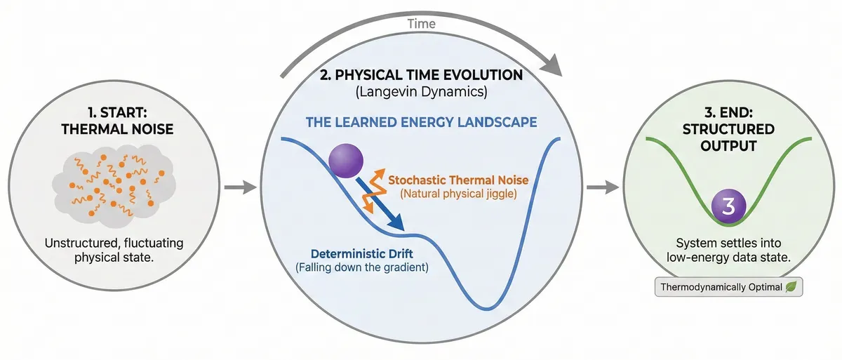
The system consists of $N$ classical, real-valued degrees of freedom $𝐱=\{x_1,x_2,...,x_N\}$. These could physically represent voltage states in electrical circuits, oscillator positions in mechanical systems, or phases in Josephson junction devices. The key is that these are fluctuating quantities whose dynamics are governed by thermal interactions with their environment.

Each degree of freedom evolves according to overdamped Langevin dynamics:

${\dot{x}}_i=-\mu \frac{\partial V_{\theta }(𝐱)}{\partial x_i}+\sqrt{2\mu k_{B}T}{\eta }_i(t)$

Let's unpack this equation:

• $\mu$ is the mobility parameter, setting the system's characteristic timescale. For existing thermodynamic hardware, ${\mu }^{-1}$ ranges from microseconds (electrical circuits) to nanoseconds (Josephson junctions).

• The first term is the deterministic drift: the system moves down the gradient of its potential energy $V_{\theta }(𝐱)$.

• The second term is the stochastic forcing: thermal fluctuations from the environment, modeled as Gaussian white noise where $⟨{\eta }_i(t)⟩=0$ and $⟨{\eta }_i(t){\eta }_j(t^{\prime })⟩={\delta }_{ij}\delta (t-t^{\prime })$.

This is the physics that governs everything from Brownian motion to the dynamics of molecules in solution. The insight is to harness it for computation.

The energy landscape

The potential energy function $V_{\theta }(𝐱)$ defines the computational landscape:

$V_{\theta }(𝐱)={\sum }_{i=1}^N(J_2{x}_i^2+J_4{x}_i^4)+{\sum }_{i=1}^N{b}_i{x}_i+{\sum }_{⟨ij⟩}{J}_{ij}{x}_i{x}_j$

Three components shape this landscape:

1. Intrinsic nonlinearity (first sum): The $J_2$ and $J_4$ terms create the basic response of each unit. With $J_4>0$, units become nonlinear—essential for the system to function as more than simple linear algebra. The quartic term also ensures thermodynamic stability as the coupling parameters are adjusted during training.

2. External biases (second sum): The $b_i$ terms are input signals applied to each unit, used to inject information into the system.

3. Pairwise couplings (third sum): The $J_{ij}$ terms couple different units together. These are the trainable parameters that will encode the learned structure—they're analogous to the weights in a neural network.

The architecture mirrors diffusion models: visible units ($N_v={28}^2=784$ for MNIST) serve as the display, while hidden units ($N_h=512$ in the demonstration) perform computation. The trainable couplings connect visible-to-hidden and hidden-to-hidden units.

Training: learning to reverse time

Here's where the physics gets beautiful. The training objective is to find couplings that allow the computer to generate the reverse of a noising trajectory.

The forward process (noising)

Start with a structured image projected onto the visible units through their biases. Set all trainable couplings $J_{ij}$ to zero. Let the system equilibrate, then run dynamics while gradually reducing the bias intensity. The image degrades into noise—this is the "noising" process familiar from diffusion models.

The reverse probability via Onsager-Machlup

The key theoretical tool is the Onsager-Machlup action, which gives the probability that a particular trajectory was generated by the Langevin dynamics.

Using a discretized Euler scheme with timestep $\Delta t$:

$x_i(t+\Delta t)=x_i(t)-\mu \frac{\partial V_{\theta }}{\partial x_i}\Delta t+\sqrt{2\mu k_{B}T\Delta t}{\eta }_i$

The displacement $\Delta x_i=x_i(t+\Delta t)-x_i(t)$ requires drawing noise values ${\eta }_i$. Inverting this relationship gives:

${\eta }_i=\frac{\Delta x_i+\mu \frac{\partial V_{\theta }}{\partial x_i}\Delta t}{\sqrt{2\mu k_{B}T\Delta t}}$

Since the ${\eta }_i$ are Gaussian with unit variance, the probability of generating a forward step $𝐱\to 𝐱+\Delta 𝐱$ is:

$P_{\theta }^{\text{step}}(\Delta 𝐱)=(2\pi {)}^{-N/2}{\prod }_{i=1}^N\exp (-{\eta }_i^2/2)$

Taking the negative log-probability:

$-\ln P_{\theta }^{\text{step}}(\Delta 𝐱)={\sum }_{i=1}^N\frac{[\Delta x_i+\mu {\partial }_i{V}_{\theta }(𝐱)\Delta t{]}^2}{4\mu k_{B}T\Delta t}$

For the reverse step ($𝐱+\Delta 𝐱\equiv {𝐱}^{\prime }\to 𝐱$):

$-\ln {\tilde{P}}_{\theta }^{\text{step}}(\Delta 𝐱)={\sum }_{i=1}^N\frac{[-\Delta x_i+\mu {\partial }_i{V}_{\theta }({𝐱}^{\prime })\Delta t{]}^2}{4\mu k_{B}T\Delta t}$

Gradient descent on couplings

To maximize the probability of generating the reverse trajectory, we sum over all steps and differentiate with respect to each parameter:

$J_{ij}\to J_{ij}+\alpha {\sum }_{k=1}^K\frac{\partial }{\partial J_{ij}}\ln {\tilde{P}}_{\theta }^{\text{step}}[\Delta 𝐱(t_k)]$

$b_i\to b_i+\alpha {\sum }_{k=1}^K\frac{\partial }{\partial b_i}\ln {\tilde{P}}_{\theta }^{\text{step}}[\Delta 𝐱(t_k)]$

The gradients can be computed analytically:

$-\frac{\partial }{\partial J_{ij}}\ln {\tilde{P}}_{\theta }^{\text{step}}=\frac{-\Delta x_i+\mu {\partial }_i{V}_{\theta }({𝐱}^{\prime })\Delta t}{2k_{B}T}{x}_j+\frac{-\Delta x_j+\mu {\partial }_j{V}_{\theta }({𝐱}^{\prime })\Delta t}{2k_{B}T}{x}_i$

$-\frac{\partial }{\partial b_i}\ln {\tilde{P}}_{\theta }^{\text{step}}=\frac{-\Delta x_i+\mu {\partial }_i{V}_{\theta }({𝐱}^{\prime })\Delta t}{2k_{B}T}$

where the energy gradient is:

${\partial }_i{V}_{\theta }(𝐱)=2J_2{x}_i+4J_4{x}_i^3+b_i+{\sum }_{j\in 𝒩(i)}{J}_{ij}{x}_j$

This is remarkably clean: the gradients depend only on local information—the displacements, forces, and neighboring unit values.

The thermodynamic interpretation: Minimizing heat

Here's where the framework connects to fundamental physics. Consider the ratio of two probabilities: the forward step probability with reference couplings ($\theta =0$) and the reverse step probability with trained couplings:

$\ln \frac{P_0^{\text{step}}(\Delta 𝐱)}{{\tilde{P}}_{\theta }^{\text{step}}(\Delta 𝐱)}\approx -\frac{\Delta Q_0+\Delta Q_{\theta }}{2k_{B}T}$

where $\Delta Q_0$ and $\Delta Q_{\theta }$ are the incremental heat dissipated by the reference and trained computers, respectively.

Integrated over an entire trajectory:

$\ln \frac{P_0[\omega ]}{P_{\theta }[\tilde{\omega }]}=-\frac{1}{2}[\beta Q_0(\omega )+\beta Q_{\theta }(\omega )]$

Training minimizes $-\ln P_{\theta }[\tilde{\omega }]$. Since the reference process is fixed, this is equivalent to minimizing $-Q_{\theta }(\omega )$, the negative heat dissipated by the denoising computer when generating the noising trajectory.

But heat changes sign under time reversal. So the learning process minimizes the heat $Q_{\theta }(\tilde{\omega })=-Q_{\theta }(\omega )$ emitted by the trained computer as it generates structure from noise.

The trained dynamics is thermodynamically optimal: it reconstructs the imposed data with minimal heat emission and entropy production. This links generative modeling directly to the second law of thermodynamics.

Numerical results

Whitelam demonstrates the framework with a digital simulation using $J_2=J_4=10k_{B}T$, 784 visible units (28×28 grid), and 512 hidden units. Training uses only three MNIST digits.

The results show:

• Independent trajectories starting from noise converge to recognizable digit structures
• The system generates diversity: different runs produce different outputs, some not in the training set
• Some outputs show "mode mixing"—expected behavior for a small-scale demonstration

The hidden units develop interpretable receptive fields—localized, digit-like structures that decompose inputs into visual components. These patterns act as the features that guide the energy landscape.

The energy efficiency argument

The thermodynamic advantage is striking. Consider the energy scales:

Digital neural network: A multiply-accumulate (MAC) operation costs ~1 pJ, or $2.4\times {10}^8{k}_{B}T$ at room temperature. A modest MLP denoiser (784→128→128→784) requires ~$2.2\times {10}^5$ MACs per step. Even with only 10 denoising steps, the energy budget exceeds $5\times {10}^{14}{k}_{B}T$.

Thermodynamic computer: The heat emitted can be calculated from the potential energy difference between trajectory start and end: $Q=V_{\theta }[𝐱(0)]-V_{\theta }[𝐱(t_f)]$. Over 1000 denoising trajectories, the mean heat emission is $⟨Q⟩=2.9\times {10}^3{k}_{B}T$ with standard deviation $3.5\times {10}^2{k}_{B}T$.

The ratio exceeds ${10}^{11}$—the thermodynamic computer would be more than 10 orders of magnitude more energy-efficient.

How this differs from Boltzmann Machines

The system resembles a nonequilibrium, continuous-spin Boltzmann machine, but with crucial differences:

Boltzmann Machine:

• Variables: Binary
• Information encoding: Equilibrium distribution
• Timing: Equilibration required
• Sampling: MCMC (simulated)

Langevin Computer:

• Variables: Continuous, real-valued
• Information encoding: Dynamical trajectories
• Timing: Physical clock, designated time
• Sampling: Natural thermal fluctuations

The Langevin computer runs on a physical clock—computation happens at a designated time without requiring equilibration. This is fundamentally different from sampling an equilibrium distribution.

What this means for hardware

If realized in analog hardware—networks of mechanical oscillators, electrical circuits, or superconducting devices—the system would:

1. Generate structured outputs by simply evolving with time under natural dynamics
2. Require no added pseudorandom noise—thermal fluctuations provide the stochasticity
3. Need no neural network guidance—the learned couplings encode all necessary information in the energy landscape

The paper notes that hybrid approaches could work too: a neural network could adjust the computer's couplings as a function of time, or set couplings to produce conditioned outputs. But the core insight is that analog hardware alone can be generative.

Open questions

Several questions remain for scaling this approach:

• Training complexity: Can this scale to the complexity of modern diffusion models? The demonstration uses only 3 digits.
• Hardware realization: What physical systems best balance the required nonlinearity, coupling adjustability, and thermal properties?
• Conditioning: How to efficiently generate specific outputs rather than sampling from the learned distribution?
• Architecture: What connectivity patterns optimize the tradeoff between expressivity and physical realizability?

The bigger picture

What strikes me about this work is how it reframes generative modeling as a question of physics rather than computation. The training process isn't just optimizing a loss function—it's finding the dynamics that minimizes entropy production. The generated outputs aren't just samples from a learned distribution—they're the thermodynamically optimal reconstructions of structured data.

This connects machine learning to a century of work on nonequilibrium statistical mechanics, opening possibilities for understanding generative models through the lens of physical law. Whether or not thermodynamic computers become practical hardware, this perspective enriches our understanding of what generation fundamentally means.